This spreadsheet activity is actually written for Google Sheets. If you are using Microsoft Excel, some of steps may be slightly different.
If you enjoy computers, you probably enjoy learning about spreadsheets. However, many of our students don’t think there is such a thing as FUN Excel activity. This one may change their minds!
You have probably seen Elf Name generators on social media. Basically you take two items unique to you, let’s say your eye color and first initial of your first name and match these with two words. This becomes your elf name.
In this version, students choose a favorite color and their hair color to get their Elf Name.
There are variations to this: your blues singer name, a band name or even something more sinister like your serial killer name. Depending on your students, you may want to mix this up.
Tasks involved in this spreadsheet:
- Vlookup formula
- Conditional formatting
- Shading cells
- Adding borders
- Data validation
- Sorting
- Merging cells
- Removing gridlines
There are a few ways you can use this in the classroom. If your students are experienced with spreadsheets, they can follow the lessons below to create this from scratch. If they are more advanced, you can just show them the finished product and challenge them to make it work. There are certainly different ways to do this. Finally, if your students are just beginning spreadsheets, just give them a copy and let them choose their own names.
(Unnecessary Warning) – Some the names on the example may be considered crude in some circles.
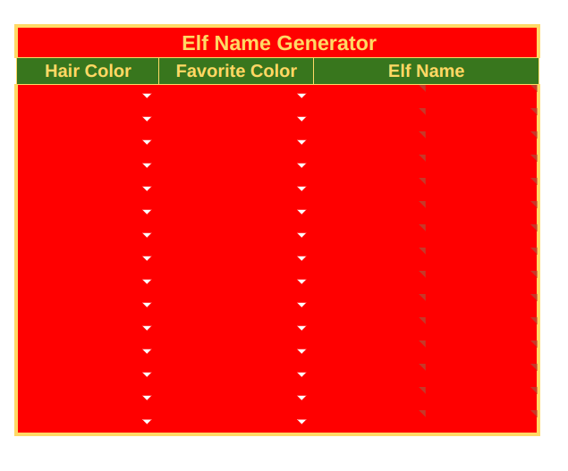
Elf Name Generator Directions
- Open a new spreadsheet.
- On the lower left hand corner, click the plus to add a second sheet to your workbook.
- Go to Sheet Two:
- In A1, type Hair Colors
- In the cells below A1, list all the hair colors you want to include
- In B1, type First Names
- In the cells below B1, type the elf first names. You will need the same amount of names as colors of hair.
- In C1, type Favorite Colors
- In the cells below C1, create a list of colors
- In D1, type Last Names
- In the cells below D1, create a list of Elf names. The C and D columns must have the same amount of entries.
- Go back to Sheet One.
- Select cells B4 to E4.
- Go to the Format menu and choose Merge Cells → Merge Horizontally.
- Type Elf Name Generator.
- Type the following:
- B5 – Hair Color
- C5 – Favorite Color
- Merge cells D5 and E5.
- In the merged cell, type Elf Name.
- Select cells B6 through B20.
- Go to the Data menu and choose Data Validation.
- The Data validation dialogue box will appear. In the second row, you will see Criteria:, List from a range and then a blank box with light gray text “e.g.Sheet1!” – click in this box.
- Click on sheet two and select the hair colors in Column A. At this point, the dialogue box will disappear and a smaller one will appear. The new box will be the Select a data range box. After you select the range, click OK. The original box will re-appear, click Save.
- On Sheet 1 you will see little down arrows in the cells below B5.
- Select cells C6 through C20.
- Go to the Data menu and choose Data Validation.
- The Data validation dialogue box will appear. In the second row, you will see Criteria:, List from a range and then a blank box with light gray text “e.g.Sheet1!” – click in this box.
- Click on sheet two and select the favorite colors in Column C. At this point, the dialogue box will disappear and a smaller one will appear. The new box will be the Select a data range box. After you select the range, click OK. The original box will re-appear, click Save.
- You should now see little arrows on the cells C6 through C20.
- In cell D6, type the following formula: =vlookup(B6,Code!$A$2:$B$11,2,False)
- Drag this formula down column to cell D20.
- In cell E6, type the following formula: =vlookup(C6,Code!$C$2:$D$12,2,False)
- Drag this formula down the column to cell E20.
- Highlight cells B4 to B20. Choose a background color. Set border and text to gold. Change cells in row 5 to green. For the steps below, we will stick to the background color of red.
- Select cells D6:D20.
- Go to the format menu and choose Conditional Formatting.
- In the Conditional format rules dialogue box:
- Under Formats cells if…
- Choose Custom formula is
- =and(C6=””)
- Under Formatting style
- Change font color to red
- Click Done
- Under Formats cells if…
- Repeat steps 26 through 28 for cells E6:E20.
- Under the view menu, click remove gridlines.
- Click on your Sheet 2 tab, select the down arrow and choose hide sheet.
- You are finished, test your results!